Reference: 수학의신.com (이상엽 선생님)
1. Matrix
1.1 Notions and Definitions
Basics
\[A = \begin{bmatrix} 1 & 2 & 3 \\ 4 & 5 & 6 \end{bmatrix}\]- elements : \(a_{ij}\) is a certain element located in i-th row and j-th column in a matrix. Here, for example, \(a_{12}\) = 2 ;
- row : (1 2 3) and (4 5 6) are called rows (there are m = 2 rows) ;
- column : (1 4), (2 5), and (3 6) are called columns (there are n = 3 columns) ;
- matrix size : A is a m(= 2) by n(= 3) matrix denoted as \( A(2 \times 3) \) or in general \( A(m \times n) \). It could also be denoted as \( A(2, 3) \) and \( A(m, n) \) ;
- transposition : the notation for transpose of the matrix A is \(A^T\) or \(A’\) and is expressed as below
Further details
\[D = \begin{bmatrix} 1 & 0 & 0 \\ 0 & 1 & 0 \\ 0 & 0 & 1 \end{bmatrix}\]- D is a diagonal matrix and (1 1 1) is the diagonal (or diagonal elements) of D ;
- D is an identity matrix which has to contain only 1 as its diagonal elements values. An identity matrix is often denoted as I ;
- D is a square matrix (number of rows = number of columns) ;
- S is a symetric matrix which has identical elememnts across the diagonal (elements in the diagnoal do not matter) ;
- A symetric is necessarily a square matrix ;
- Transpose of a symetric matrix is equal to its original matrix \(S^T = S\) ;
1.2 Matrix Computation
For \(A(m \times n) = (a_{ij} \) and \(B(m \times n) = (b_{ij}) \), following computations are valid
- Addition and Substration : \( A ± B = (a_{ij} ± b_{ij}) \) ;
- Constant factor multiplication : \( cA = (ca_{ij}) \) (c is a constant) ;
For \(A(m \times n) = (a_{ij} \) and \(B(n \times r) = (b_{jk}) \), following computations are valid
- Matrix multiplication : \( A(m \times n) \times B(n \times r) = AB(m \times r) = (c_{ik}) = \sum_{j=1}^n{a_{ij}b_{jk}} \) ;
- Matrix multiplication computation is not commutative. Which means \(AB ≠ BA\) ;
Example : to be updated
2. First Order Equation System
2.1 Another way to express a matrix
A first order equation system (FOES) is another way to express and solve a matrix problem. Reciprocally, we can also express a FOSE in terms of matrix and solve it with matrices through two different ways. The first method is Gauss-Jordan elimination method,
2.1.1 Gauss-Jordan Elimination Method
First we express the given FOES as an augmented matrix,
\[\begin{cases} x + 2y = 5 \\ 2x + 3y = 8 \end{cases} \iff \begin{bmatrix} 1 & 2 & 5 \\ 2 & 3 & 8 \end{bmatrix}\]then we use one of or a combination of following operations to simplify the matrix as much as possible in a echelon shape :
- multiply a constant to a row ;
- add/substract the result of (1) to/from another row ;
- switch rows ;
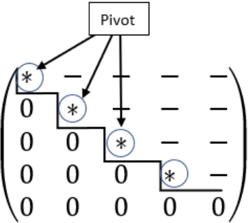
The final matrix is called reduced row echelon matrix due to its form. With Gauss-Jordan elimination method, we are supposed to simplify all the elements to zeros, ones or if impossible, to prime numbers.
The final matrix then can be expressed in FOES as below
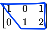
\[\begin{bmatrix} 1 & 0 & 1 \\ 0 & 1 & 2 \end{bmatrix} \implies \begin{cases} 1x + 0y = 1 \\ 0x + 1y = 2 \end{cases} \implies \begin{cases} x = 1 \\ y = 2 \end{cases}\]The solutions that this method found are \(x = 1\) and \( y = 2\).
the second method is Inverse matrix method.
2.1.2 Inverse Matrix Method
Before applying this method, there are two questions to answer. “How do we know if the inverse matrix exists ?” and then “If it does, how do we compute it ?”. These questions will be answered in the section 3. However the computation is done as following
For a matrix equation \(AX = B\), if \(A\)’s inverse matrix \(A^{-1}\) exists, then \(X = A^{-1}B\),
(coefficient matrix)(variable vector/matrix) = (solution vector/constant matrix) :
\[\begin{bmatrix} 1 & 2 \\ 3 & 4 \end{bmatrix} \begin{bmatrix} x \\ y \end{bmatrix} = \begin{bmatrix} 5 \\ 8 \end{bmatrix} \iff \begin{bmatrix} x \\ y \end{bmatrix} = \begin{bmatrix} 1 & 2 \\ 3 & 4 \end{bmatrix}^{-1} \begin{bmatrix} 5 \\ 8 \end{bmatrix}\]3. Determinant
3.1 Definition
A determinant is a function that transforms a matrix into a constant.
For a matrix A, determinant is computeted differently according to matrix size :
- \( A(0 \times 0) \) : \( \det(A) = 0 \)
- \( A(1 \times 1) \) : \( \det(A) = a \)
- \( A(2 \times 2) \) : \( \det(A) = a_{11}a_{22} - a_{12}a_{21} \)
- \( A(3 \times 3) \) : \( \det(A) = a_{11}M_{11} - a_{12}M_{12} + a_{13}M_{13} \)
- \( A(4 \times 4) \) : \( \det(A) = a_{11}M_{11} - a_{12}M_{12} + a_{13}M_{13} - a_{14}M_{14} \)
Minor Matrix
A minor matrix \(M_{ij}\) is a determinant of a submatrix from a matrix \(A(n \times n)\) where \(n>i,j\). The submatrix concerning \(M\) is matrix \(A\) without \(i^{th}\) row and \(n^{th}\) column.
example)
\[A = \begin{bmatrix} a_{11} & a_{12} & a_{13} \\ a_{21} & a_{22} & a_{23} \\ a_{31} & a_{32} & a_{33} \end{bmatrix} ~~~~~~~~~~ M_{11} = \begin{vmatrix} a_{22} & a_{23} \\ a_{32} & a_{33} \end{vmatrix}\]Sarrus Rule
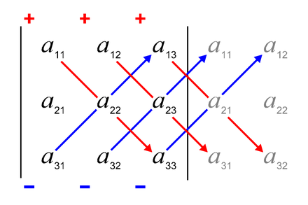
Sarrus Rule is a mnemonic device for computing the determinant of \(3 \times 3\) matrix named after French mathematician Pierre Frédéric Sarrus. Consider \(A(3\times 3)\). \(\det(A)\) is computeted by the following rule :
Cofactor
A cofactor is an element that constitues an inverse matrix. It can be computeted from minor matrix.
\[c_{ij} = (-1)^{i+j}M_{ij}\]3.2 Inverse Matrix
For a matrix A, its inverse matrix is defined as below :
\[A^{-1} = \frac{1}{\det(A)}\begin{bmatrix} c_{11} & c_{21} & \ldots \\ c_{11} & c_{22} & \ldots \\ \vdots & \vdots & \ddots \end{bmatrix}\](note that cofactor indexes are transposed)
This definition answers two questions in the section 2. By the property of fraction, \(\det(A)\) cannot be 0. So if \(\det(A)\) is not equal to 0, then we can compute \(A^{-1}\), therefore we can know if \(A^{-1}\) exists or not by checking the value of \(\det(A)\). Once it is verified, we can compute the definition formula of \(A^{-1}\).
Why the inverse matrix is defined as above ?
Just like \(a \cdot a^{-1} = 1 \), for any matrix, \(A \cdot A^{-1} = I \). The demonstration is as following :
Consider a matrix \(A(n,n)\).
\[\begin{bmatrix} a_{11} & a_{12} & \ldots & a_{1n} \\ a_{21} & a_{22} & \ldots & a_{2n} \\ \vdots & \vdots & \ddots & \vdots \\ a_{n1} & a_{n2} & \ldots & a_{nn} \\ \end{bmatrix} \begin{bmatrix} c_{11} & c_{21} & \ldots & c_{n1} \\ c_{12} & c_{22} & \ldots & c_{n2} \\ \vdots & \vdots & \ddots & \vdots \\ c_{1n} & c_{2n} & \ldots & c_{nn} \\ \end{bmatrix} = \begin{bmatrix} |A| & 0 & \ldots & 0 \\ 0 & |A| & \ldots & 0 \\ \vdots & \vdots & \ddots & \vdots \\ 0 & 0 & \ldots & |A| \\ \end{bmatrix}\] \[\begin{align} & \iff A \cdot adj(A) = |A|\\ & \iff A \cdot \frac{1}{|A|} \cdot adj(A) = I\\ & \iff A \cdot A^{-1} = I \end{align}\]This demonstration gives the definition of the inverse matrix \( A^{-1} = \frac{1}{|A|}adj(A) \). In the definition, we can see that \( |A| \) is in the denominator. Therefore, \( \det(A) \equiv |A| \) cannot be equal to 0. As a corollary, we can say that if \( \det(A) \) is equal to 0, then \( A \) doesn’t have the inverse matrix. So this becomes the very first thing to verify before proceeding to compute the inverse matrix of any matrix.
Example : inverse matrix
Consider a matrix \( A(2,2) \) :
\[A \cdot adj(A) = |A|\] \[\begin{align} & \iff \begin{bmatrix} a_{11} & a_{12} \\ a_{21} & a_{22} \end{bmatrix} \begin{bmatrix} c_{11} & c_{21} \\ c_{12} & c_{22} \end{bmatrix} = \begin{bmatrix} |A| & 0 \\ 0 & |A| \end{bmatrix} \\ & \iff \begin{bmatrix} 1 & 2 \\ 3 & 4 \end{bmatrix} \begin{bmatrix} 4 & -2 \\ -3 & 1 \end{bmatrix} = \begin{bmatrix} -2 & 0 \\ 0 & -2 \end{bmatrix} \\ & \iff \begin{bmatrix} 1 & 2 \\ 3 & 4 \end{bmatrix} \frac{1}{-2} \begin{bmatrix} 4 & -2 \\ -3 & 1 \end{bmatrix} = \begin{bmatrix} 1 & 0 \\ 0 & 1 \end{bmatrix} \end{align}\] \[\implies A^{-1} = \frac{1}{-2} \cdot \begin{bmatrix} 4 & -2 \\ -3 & 1 \end{bmatrix}\]3.2.1 Conclusion
Now we know how to verify if \( A^{-1} \) exists and how to compute it. But what we really have to know in the end is \( X = A^{-1}B \). Computing \( X \) is just same as computing any matrix multiplication. But what if we only wanna know a certain element of X ?. For instance, what if we only wanna know \( x_{12} \) from \( X \) ?
In this case, we use Cramer Rule, also called Carmer’s algorithm.
3.3 Cramer Rule
For a matrix equation \( AX = B \) in which A has a non null determinant, \( j = 1, \ldots, n \)
\[x_j = \frac{\det (A_j)}{\det (A)} = \frac{\begin{vmatrix} a_{11} & \ldots & b_1 & \ldots & a_{1n} \\ a_{21} & \ldots & b_2 & \ldots & a_{2n} \\ \vdots & & \vdots & & \vdots \\ a_{n1} & \ldots & b_n & \ldots & a_{nn} \end{vmatrix}} {\begin{vmatrix} a_{11} & \ldots & a_{1j} & \ldots & a_{1n} \\ a_{21} & \ldots & a_{2j} & \ldots & a_{2n} \\ \vdots & & \vdots & & \vdots \\ a_{n1} & \ldots & a_{nj} & \ldots & a_{nn} \end{vmatrix}}\]where \(A_j\) is a matrix A whose \(j^{th}\) column is replaced by the vector B.