Regression with Panel Data
1. Panel Data
Panel data or longitudinal data is a data structure that records data for n different entities observed at T different time periods. We distinguish between:
- balanced panel: each entity coupled with each time period (missing data could exist but every data is coupled between entity and time)
- unbalanced panel: at least one entity in one time period missing
Let’s take an example of fatalities dataset: collected data on traffic fatalities in the U.S. Entities are the 48 U.S states recorded for 7 years, from 1982 to 1988. It is a balanced panel.
2. Regression with Panel Data
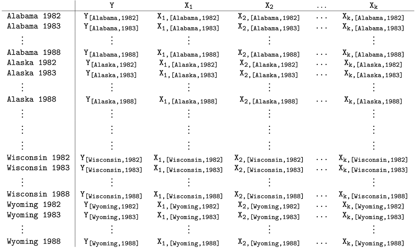
The multi-variable regression model (MRM) in case of a panel data structure with I entities and T time periods in scalar form reads
\[Y_{it} = \beta_0 + \beta_1 X_{(1,it)} + \beta_2 X_{(2,it)} + \cdots + \beta_k X_{(k,it)} + u_{it}\]with \(i = 1, \cdots, I \) and \(t = 1, \cdots, T\).
In matrix form it remains
\[\mathbf{Y} = \mathbf{X}\beta + \mathbf{u}\]but now Y and u are two \( (IT \times 1) \) sized vectors, X a \( (IT \times (K+1)) \) sized matrix and \(\beta\) is a \( ((K+1)\times 1) \) sized vector.
Let’s take an example. Suppose we study how effective various government policies (e.g tax on beer) designed to discourage drunk driving are in reducing traffic deaths.
Since we do not know what to do with observations in different years, we estimate the following regression model of two different time periods
\[FATAL_{it} = \beta_0 + \beta_1 BTAX_{it} + u_{it}\]where \(i = 1, \cdots, 48 \) with \(t=1982\) and \(t=1988\). Meaning we consider all the 48 states but only the first and the last years. the regression results in R gives us
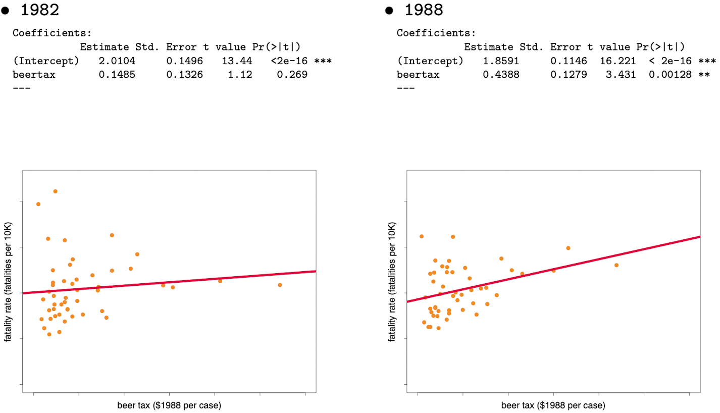
As we can see, estimated beertax coefficient in 1982 is statistically insignificant (high p-value) and the one in 1988 is statistically significant (low p-value). How come this happens? Should we trust these results?
The answer is No. Indeed, there can be a substantial omitted variable bias. Many factors affect the fatality rate such as
- quality of automobiles;
- maintenance of highways;
- driving in rural or urban areas;
- density of cars;
- social acceptability of “drink and drive” etc.
Any of these factors may be correlated with alcohol tax, and if they are, they will lead to an OVB problem. Unfortunately, not all of these variable can be (properly) measured. So? What do we have to do?
Imagine a new regression model
\[FATAL_{it} = \beta_0 + \beta_1 BTAX_{it} + \beta_2 Z_i + u_{it}\]where \(Z_i\) represents a potentially dangerous omitted variable that is heterogeneous across states but does not change in time (no t) or it changed very very slowly.
Following the new model, in 1982 and 1988, we will get
\[\begin{align} & A:FATAL_{i,1988} = \beta_0 + \beta_1 BTAX_{i,1988} + \beta_2 Z_i + u_{i,1988} \\ & B:FATAL_{i,1982} = \beta_0 + \beta_1 BTAX_{i,1982} + \beta_2 Z_i + u_{i,1982} \end{align}\]To assess the change in each state between 1988 and 1982, we do \( A - B \):
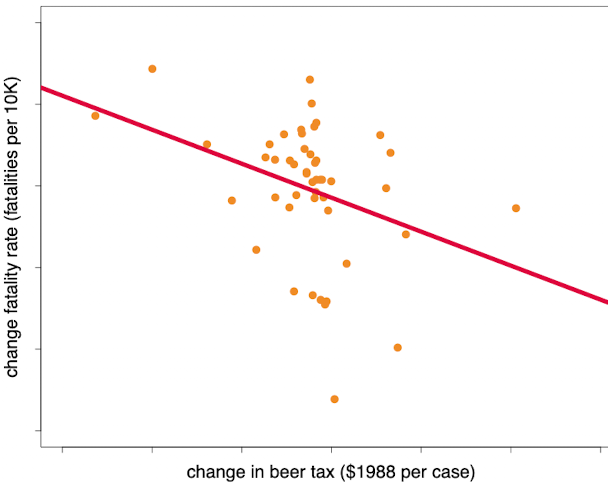
\[C:FATAL_{i,1988} - FATAL_{i,1982} = \beta_1(BTAX_{i,1988} - BTAX_{i,1982}) + (u_{i,1988} - u_{i,1982})\]Note that \(Z\) has now disappeared. Therefore its effect has disappeared as well. We obtained an interesting new model, called model in differences.
If we regress this model, we get the following result
![]()
Interpretation
- All factors that have not changed between 1982 and 1988 cannot drive a change in fatality rate between 1982 and 1988. Taking the difference controls for any factor constant over time
- The intercept is the change in fatality rate in absence of a change in beer tax.
- Beer tax change coefficient -1.04 means an increase in beer tax by 1$ reduces 1.04 fatalities per 10K people. This is very large given the average fatality rate is 2.
3. Fixed Effects Model
The fixed effects regression model
- is a method for controlling for omitted variables in panel data that vary across entities (states in our example) but do not change over time;
- has n intercepts, one for each entity.
3.1 Model
Consider the following regression model
\[\begin{align} Y_{it} &= \beta_0 + \beta_1 X_{it} + \beta_2 Z_{i} + u_{it} \\ &= (\beta_0 + \beta_2 Z_i) + \beta_1 X_{it} + u_{it} \\ &= \alpha_i + \beta_1 X_{it} + u_{it} \end{align}\]where \(Z_i\) is an unobserved variable that varies across i but does not change over time. Since it does not vary, we can fix the effect \(\alpha_i = (\beta_0 + \beta_2 Z_i)\) and interpret our regression model as having n different intercepts, one for each i.
Let’s go back to our previous example. With our new fixed effects regression model, the panel data will look like
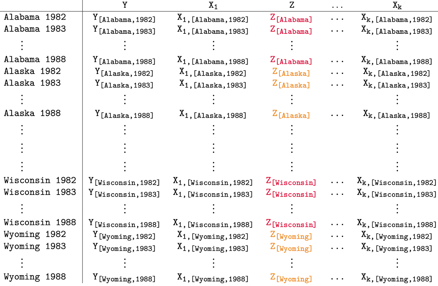
Let’s focus on Alaska
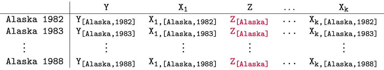
This would imply that there remains only one source of variability according to the time variability and Z plays the role of a country specific constant (not a state specific constant).
3.2 Limits
Note that panel data encompasses data coming from several entities. So this is a pool of data. And when we introduced \(Z_i\), we said that it represents a potentially dangerous omitted variable that is heterogeneous across states. Therefore, we could replace \((\beta_0 + \beta_2 Z_i)\) by a fixed effect denoted \(\alpha_i\) proper to each state. What is the consequence of the combination of pool of data and fixed effect?
Let’s discuss with an example.
Consider an artificial dataset with 750 observations generated as follows
\[Group~1:~ Y_i = -20 + X_i + u_i ~~~~~where~~ \begin{cases} \beta_0 = -20 \\ \beta_1 = 1 \\ n.obs = 250 \end{cases}\] \[Group~2:~ Y_i = X_i + u_i ~~~~~where~~ \begin{cases} \beta_0 = 0 \\ \beta_1 = 1 \\ n.obs = 250 \end{cases}\] \[Group~3:~ Y_i = 20 + X_i + u_i ~~~~~where~~ \begin{cases} \beta_0 = 20 \\ \beta_1 = 1 \\ n.obs = 250 \end{cases}\] \[Pool:~ Y_i = X_i + u_i ~~~~~where~~ \begin{cases} \beta_0 = 0 \\ \beta_1 = 1 \\ n.obs = 250 \end{cases}\]Using the “Pooled data”, you estimate the model \( Y_i = X_i + u_i \) obtaining the following results:
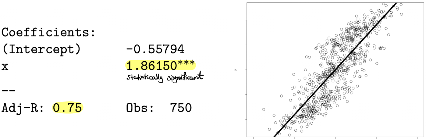
Is everything ok here? Not at all.
Indeed when we estimate the same model group by group, we will have different results
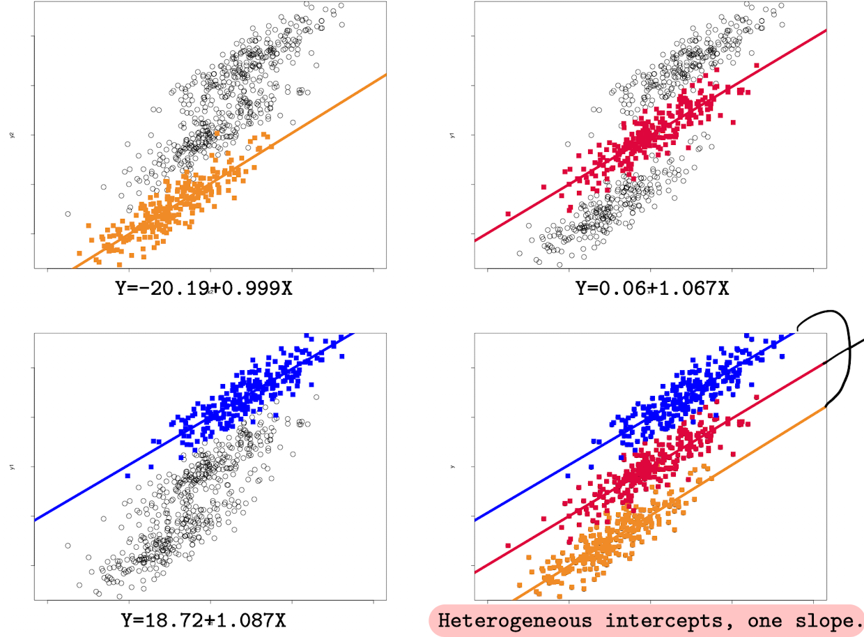
We can see that in the last graph, regression functions are parallel, sharing one same slope, and heterogeneous(different) intercepts.
But if we pool the three groups and do regression on it, the OLS estimator on the pooled dataset performs badly!
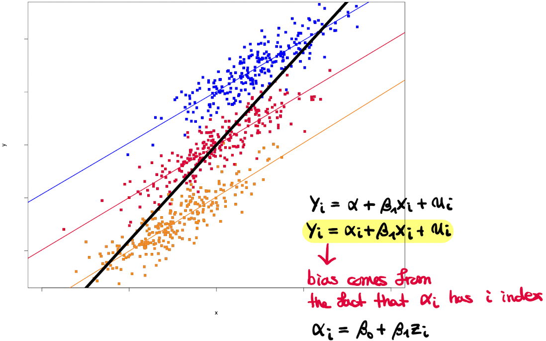
The OLS estimator suffers from an unobserved heterogeneity bias.
But don’t worry, there are solutions to this kind of problem. One of them is the Least Squares Dummy Variable Model (LSDV).
4. Least Squares Dummy Variable Model (LSDV)
The FE regression model
\[Y_{it} = \beta_1 X_{it} + \alpha_i + u_{it}\]can be eqauivalently written in terms of a set of dummy variables (with our example, there will be 48 dummy variables)
\[Y_{it} = \beta_1 X_{it} + \gamma_2 D_2 + \cdots + \gamma_n D_n + u_{it}\]where we have skipped \(D_1\) to avoid the dummy variable trap (multicolinearity between independent variables).
FERM and LSDV are mathematically equivalent. But LSDV allows heterogeneity of intercepts.
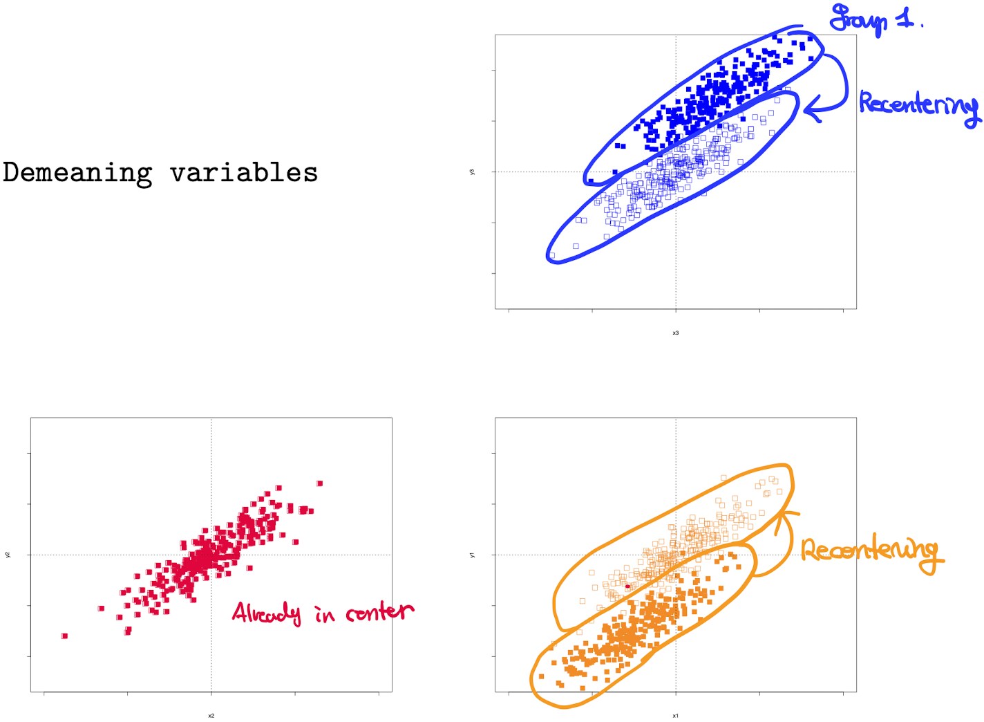
5. Fixed Effects Model - within transformation
Consider again the model
\[Y_{it} = \beta_1 X_{it} + \alpha_i + u_{it}\]and take the average of both side of the equation
\[\overline{Y}_{i} = \beta_1 \overline{X}_{i} + \alpha_i + \overline{u}_{i}\]where \( \overline{Y}_ i = \frac{1}{T} \sum Y_{it} \), \( \overline{X}_i \) and \( \overline{u}_i \) are defined similarly and clearly, \(\overline{\alpha}_i = \alpha_i\).
Then taking the difference from the original model, we get
\[\begin{align} Y_{it} - \overline{Y}_{i} &= \beta_1 (X_{it} - \overline{X}_{i}) + (\alpha_i - \alpha_i) + u_{it} - \overline{u}_{i} \\ &= \beta_1 ( X_{it} - \overline{X}_i ) + u_{it} - \overline{u}_i \end{align}\]Then we obtain a Within Transformed Fixed Effects Model
\[\begin{align} & Y_{it} - \overline{Y}_{i} = \beta_1 ( X_{it} - \overline{X}_i ) + u_{it} - \overline{u}_i \\ \iff & \widetilde{Y}_{it} = \beta_1 \widetilde{X}_{it} + \widetilde{u}_{it} \end{align}\]where we have eliminated the unobserved heterogeneity in intercepts, and as a consequence, the OLS estimators are unbiased.
Graphically this looks like
The result in the pooled group looks like
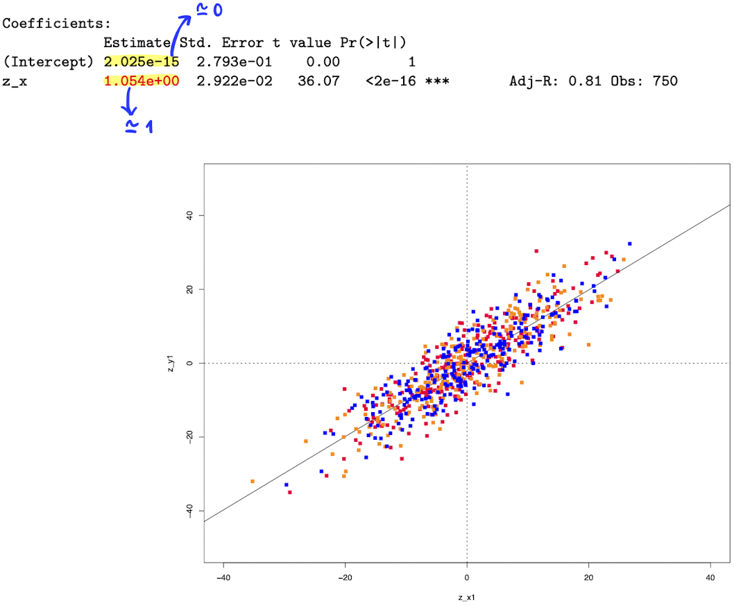
Clearly heterogeneity bias has been removed.