Non-Linear Regression Functions
1. Introduction
Two types of non-linearity in regression functions:
- Non-linear functions of a single independent varialbe (most prevailing type)
- Polynomials
- Logarithms
- Interactions
- (these 3 types are all eligible for OLS estimation)
- Regression functions that are non-linear in the parameters (only a sketch here)
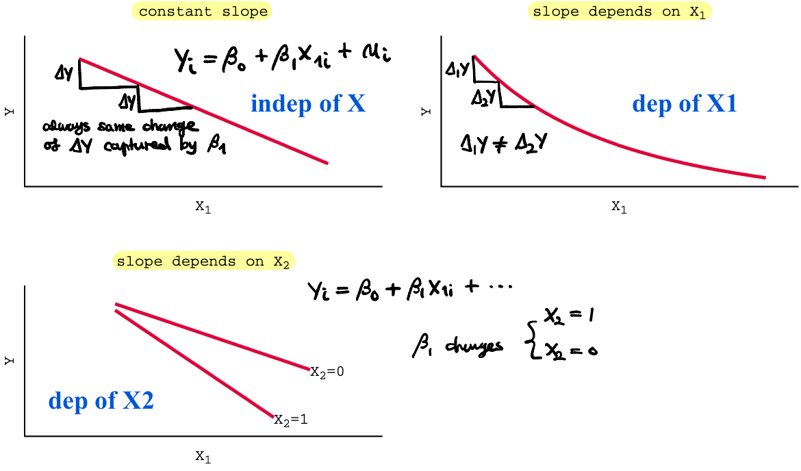
We are going to study 2 groups of methods useful when
- the relation between \(X_1\) and \(Y\) depends on the value of \(X_1\) itself;
- the relation between \(X_1\) and \(Y\) depends on the value of \(X_2\)
examples)
1.1 General Approach
In general, the population regression function reads
\[Y_i = f(X_{1i}, \cdots, X_{ni}) + u_i~~~~~i=1,\cdots,n\]where f can be a linear or non-linear function.
In the population, the effect on Y of a change in \(X_1\), \(\Delta X_1\) is:
- \(\beta_1 \Delta X_1 ~\) if f is linear;
- \( f(X_{1i}+\Delta X_{1i}, X_{2i}, \cdots, X_{ni} ) - f(X_{1i}, X_{2i}, \cdots, X_{ni})~ \) if f is non linear
Since this is a population regression function, of course, both \(\beta_1\) and \(f\) are unknown and need to be estimated by \(\hat{\beta}_1\) and \(\hat{f}\).
1.2 Modeling Non-Linearities
- Identify a possible non-linear relation based on the underlying economic theory;
- Specify a non-linear function and estimate its parameters by OLS method;
- Determine if the non-linear model improves upon a linear model;
- Plot the estimated non-linear regression function (if possible);
- Estimate the effect on Y of a change in X.
1.3 Notation
How to estimate the effect on Y of a change in X? by measuring the elasticity.
The elasticity of Y with respect to X is
\[E \equiv \frac{\frac{\Delta Y}{Y}}{\frac{\Delta X}{X}} = \frac{X}{Y}\frac{\Delta Y}{\Delta X}\]E gives us the percentage points change of Y associated with a 1% increase in X.
Note Bene
Going from 10% to 11% is either a 1 percentage point increase or 10% increase. It is not a 1% increase.
2. Polynomial Regression
Before getting into it, polynomial specification of non-linear regression function is not frequently used in econometrics modeling.
This is the first way to specify a non-linear regression for \(X_1\) using a polynomial in \(X_1\):
\[Y = \beta_0 + \beta_{11}X_1 + \beta_{12}X^2_1 + \cdots + \beta_{1r}X^r_1 + u\]- Obviously this model is easily estimatable with OLS (in R, lm(y ~ X + X^2 + …))
- With r = 2 and r = 3 we obtain the quadratic and cubic regression models (r = 3 happens almost never)
- Using the F-test and the t-test, you can test hypothesis on the linear vs polynomial nature of the population regression function: \( H_0:\beta_{12}=0
vsH_1:\beta_{12}≠0\) - Interpreting coefficients in a polynomial regression function is not trivial, the best is to plot the function and compute the estimated effect on Y of a change in \(X_1\) for different values of \(X_1\).
Let’s take a simple example.
2.1 Quadratic Regression
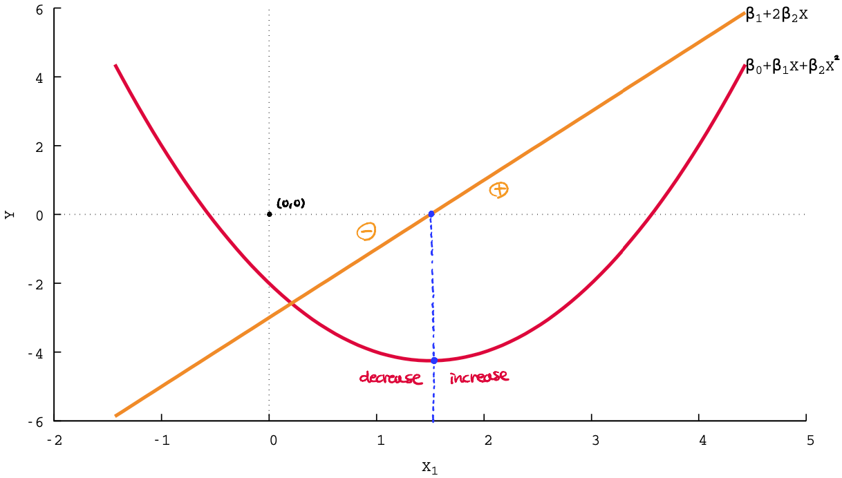
\[Y_i = \beta_0 + \beta_1 X_{1i} + \beta_2 X^2_{1i} + u_i\]- \(\beta_1\) cannot be anymore the effect on Y of a change of \(X_1\) holding \(X^2_1\) constant.
- the effect on Y of a change in \(X_1\) is indeed given by
this depends on the value of \(X_1\).
example)
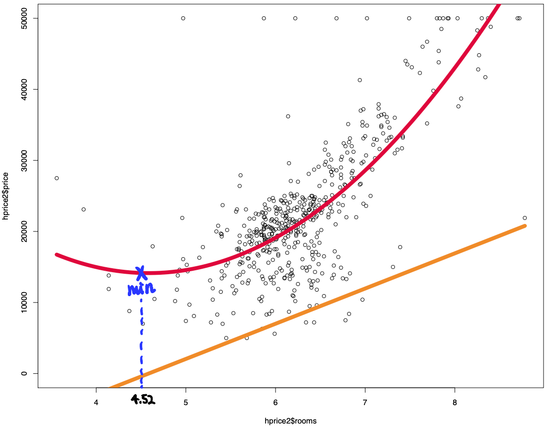
We can think of this kind of regression:
\[Price_i = \beta_0 + \beta_1 Nrooms_i + \beta_2 Nrooms^2_i + u_i\]Real result:
3. Logarithmic Regression
This is the second way to specify a non-linear regression for \(X_1\) using logarithms in \(X_1\). This is one of the most used models of non-linear regression function.
3.1 Notation
Given a model like
\[\ln(Y) = \beta_0 + \beta_1 \ln(X)\]we have to consider the following things
- \(\ln(Y + \Delta Y) - \ln(Y)\) is the logarithmic difference
- \( \frac{\Delta \ln(Y)}{\Delta \ln(X_1)}\) is the log derivative of Y as a function of \(X_1\)
- These are the two important relations:
- if \(\Delta Y / Y \approx 0\) then \( \log(Y + \Delta Y) - \log(Y) \approx \Delta Y / Y \)
- elasticity of Y wrt \(X_1\): \( \frac{\Delta \log(Y)}{\Delta \log(X_1)} = \frac{\Delta Y / Y}{\Delta X_1 / X_1} = \frac{\Delta Y X_1}{\Delta X_1 Y} \)
In the case of logarithmic regression, interpretation for elasticity changes depending on the type of logarithmic regression. There are three types of logarithmic regression function:
- \(Y\) and \(\log(X)\): linear-log model
- \(\log(Y)\) and \(X\): log-linear model
- \(\log(Y)\) and \(\log(X)\): log-log model
3.2 Linear-Log Model
First type of logarithmic regression model is linear-log model that reads
\[Y_i = \beta_0 + \beta_1 \log(X_i) + u_i\]The effect on Y of a change in X is captured by:
\[\begin{align} \Delta Y(X) &= \frac{\Delta Y(X)}{\Delta \log(X)} \times \frac{\Delta \log(X)}{\Delta X} \Delta X \\ &= \beta_1 \frac{\Delta X}{X} \end{align}\]where
- \(\frac{\Delta Y(X)}{\Delta \log(X)}\) captures the change in Y depending on the change in \(\log(X)\) (bc Y depends on \(\log(X)\));
- \(\frac{\Delta \log(X)}{\Delta X}\) captures the change in \(\log(X)\) depending on the change in X (bc \(\log(X)\) depends on X);
- Lastly \(\Delta X\) is multiplied becaused everything, in the end, depends on X.
Hence we can use the following measure
\[\Delta Y(X) = \beta_1 \frac{\Delta X}{X} = \frac{\beta_1}{100}\frac{\Delta X}{X}100\]which implies that a change of X by 1% is associated with an absolute change in Y of \(\frac{\beta_1}{100}=0.01\beta_1\).
3.3 Log-Linear Model
Second type of logarithmic regression model is log-linear model that reads
\[\log(Y_i) - \beta_0 + \beta_1X_i + u_i\]The effect on Y of a change in X is captured by:
\[\begin{align} \Delta Y(X) &= \frac{\Delta Y(X)}{\Delta \log(X)} \times \frac{\Delta \log(X)}{\Delta X} \Delta X \\ &= \left( \frac{\Delta \log(X) }{\Delta Y(X)} \right)^{-1} \times \frac{\Delta \log(X)}{\Delta X} \Delta X \\ &= \left( \frac{1}{Y} \right)^{-1} \times \frac{\Delta \log(X)}{\Delta X} \Delta X \\ &= \beta_1 Y \Delta X \end{align}\]Hence we can use the following measure
\[\frac{\Delta Y(X)}{Y}100 = 100 \beta_1 \Delta X\]which implies that a marginal change of X is associated with a change in Y of \([100 \beta_1]\% \).
3.4 Log-Log Model
Third type of logarithmic regression model is log-log model that reads
\[\log(Y_i) = \beta_0 + \beta_1 \log(X_i) + u_i\]The effect on Y of a change in X is captured by:
\[\begin{align} \Delta Y(X) &= Y \frac{\Delta \log(Y)}{\Delta \log(X)} \frac{\Delta \log(X)}{\Delta X} \Delta X \\ &= \beta_1 \frac{Y}{X} \Delta X \end{align}\]Hence we can use the following measure
\[\frac{\Delta Y}{Y}100 = \beta_1 \frac{\Delta X}{X} 100\]which implies that a change of 1% of X is associated with a change in Y of \(\beta_1\)%. \(\beta_1\) is an elasticity.
3.5 Elasticity Summary
In general, when reporting results, elasticities should be preferred since they are easier to interpret and to be compared.
| Case | Regression Models | Elasticity of \(E[Y/X]\) wrt X |
|---|---|---|
| Linear | \(Y = \beta_0 + \beta_1 X \) | \(\frac{\beta_1 X}{\beta_0 + \beta_1 X}\) |
| Linear-Log | \(Y = \beta_0 + \beta_1 \log(X) \) | \(\frac{\beta_1 }{\beta_0 + \beta_1 \log(X)}\) |
| Log-Linear | \(\log(Y) = \beta_0 + \beta_1 X \) | \(\beta_1 X \) |
| Log-Log | \(\log(Y) = \beta_0 + \beta_1 \log(X) \) | \(\beta_1 \) |
4. Interaction Regression
This is the third way to specify a non-linear regression using interactions between dummy variables. This is one of the most used models, with logarithmic models, of non-linear regression function.
Consider the following population regression model
\[Y_i = \beta_0 + \beta_1 D_{1i} + \beta_2 D_{2i} + u_i\]where \(D_1\) and \(D_2\) are two binary variables. An important limitation of this model is that \(\beta_1\), the effect on Y of a switch from 0 to 1 of \(D_1\), does not depend on the value of \(D_2\). This means Y will only have separate effect of \(D_1\) and \(D_2\).
4.1 Interaction Model - Two Dummy Variables
An easy extension to allow interaction between \(D_1\) and \(D_2\) is
\[Y_i = \beta_0 + \beta_1 D_{1i} + \beta_2 D_{2i} + \beta_3(D_{1i} \times D_{2i}) u_i\]where \( (D_{1i} \times D_{2i}) \) is called interaction term.
example)
It is somewhat tricky to interpret the coefficients of such model. Let’s take a precise exmaple.
Consider the following model in the U.S.
\[SCORE_i = \beta_0 + \beta_1 Hi\_STR_i + \beta_2 Hi\_ENG_i\]where
- Hi_STR is high student to teacher ratio in state i. If equal to 1, student-teacher ratio is high (bad), otherwise (good) 0;
- Hi_ENG is high english learner percentage in state i. If equal to 1, high number of english learner (bad), otherwise (good) 0.
Using the three coefficients, we can build the following 4 possibilities of combination:
- \(\beta_0 = SCORE(Hi’STR_i=0 ~;~ Hi’ENG_i=0 ) \),
- \(\beta_0 + \beta_1 = SCORE(Hi’STR_i = 1 ~;~ Hi’ENG_i = 0 ) \),
- \(\beta_0 + \beta_2 = SCORE(Hi’STR_i = 0 ~;~ Hi’ENG_i = 1 ) \),
- \(\beta_0 + \beta_1 + \beta_2 = SCORE(Hi’STR_i = 1 ~;~ Hi’ENG_i = 1 ) \).
Let’s say we got the following results
| testscr | Coef. | Std.Err. |
|---|---|---|
| \(\beta_1\) | -3.586 | 1.610 |
| \(\beta_2\) | -19.718 | 1.601 |
| \(\beta_0\) | 664.725 | 1.200 |
where the effect on the test score of moving from a low to high student-teacher ratio is the same for states with high or low percentage of english learners.
Let’s now introduce the interaction terms that transform the model in
\[SCORE_i = \beta_0 + \beta_1 Hi\_STR_i + \beta_2 Hi\_ENG_i + \beta_3 (Hi\_STR_i \times Hi\_ENG_i)\]where
- (Hi_STR \(\times\) Hi_ENG) is high student to teacher ratio and high english lerner percentage in state i. If equal to 1, both factors are high, otherwise 0;
Using the three coefficients, we can build the following 4 possibilities of combination:
- \(\beta_0 = SCORE(Hi’STR_i=0 ~;~ Hi’ENG_i=0 ) \),
- \(\beta_0 + \beta_1 = SCORE(Hi’STR_i = 1 ~;~ Hi’ENG_i = 0 ) \),
- \(\beta_0 + \beta_2 = SCORE(Hi’STR_i = 0 ~;~ Hi’ENG_i = 1 ) \),
- \(\beta_0 + \beta_1 + \beta_2 + \beta_3 = SCORE(Hi’STR_i = 1 ~;~ Hi’ENG_i = 1 ) \).
In this case, the effect on the test core of moving from a low to a high student-teacher ratio can depend on the percentage of english learners present in the district.
In this case, we will have the following results of OLS estimates
| testscr | Coef. | Std.Err. |
|---|---|---|
| \(\beta_1\) | -1.907 | 2.233 |
| \(\beta_2\) | -18.162 | 2.150 |
| \(\beta_3\) | -3.494 | 3.222 |
| \(\beta_0\) | 664.143 | 1.314 |
Moving from a low student-teacher ratio state to a high student-teacher ratio state implies an effect on test scores:
- -1.90 if the fraction of english learners is low,
- -1.90 and -3.50 if the fraction of english learners is high (there is a combined effect).
4.2 Interaction Model - One Dummy & One Continuous Variable
In case of an interaction between a continuous and a dummy variable, the regression model can be written as
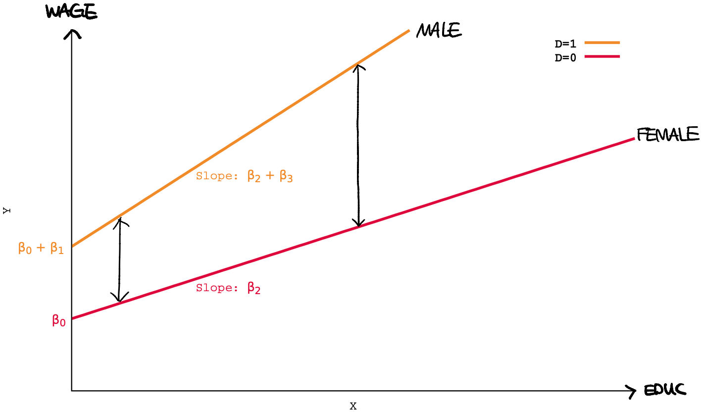
\[Y_i = \beta_0 + \beta_1 D_i + \beta_2 X_i + \beta_3 (D_i \times X_i) + u_i\]The easiest way to interpret this model is to note that it contains two different regression models depending on the value of \(D_i\) which can be separated into two sub-models:
\[\begin{cases} Y_i = \beta_0 + \beta_2 X_i + u_i~~~~~~~~~~~~~~~~~~~~~~~~~~~when D_i = 0\\ Y_i = (\beta_0 + \beta_1) + (\beta_2 + \beta_3)X_i + u_i~~~~when D_i = 1 \end{cases}\]example)
4.3 Interaction Model - Two Continuous Variables
In case of an interaction between two continuous variables, the regression model can be written as
\[Y_i = \beta_0 + \beta_1 X_{1i} + \beta_2 X_{2i} + \beta_3 (X_{1i} \times X_{2i}) + u_i\]the intuition remains the same. The effects on Y of a change in \(X_1\), holding \(X_2\) constant, and of a change in \(X_2\), holding \(X_1\) constant are
\[\begin{align} \Delta Y &= (\beta_1 + \beta_3 X_2) \Delta X_1 \\ \Delta Y &= (\beta_2 + \beta_3 X_1) \Delta X_2 \end{align}\]and we can interpret \(\beta_3\) as the effect on Y of a unit increase of \(X_1\) and \(X_2\) above and beyond the sum of the effects of a unit increase of \(X_1\) alone and of \(X_2\) alone.
Indeed the effects on Y of a simultaneous change in \(X_1\) and \(X_2\) are
\[\Delta Y = (\beta_1 + \beta_3 X_2)\Delta X_1 + (\beta_2 + \beta_3 X_1) \Delta X_2 + \beta_3 \Delta X_1 \Delta X_2\]5. Non Linearities in Paramaeters
The linear OLS problem was written as
\[\min_{\beta} \sum (Y_i - \beta_0 - \beta_1 X_{1i} - \cdots - \beta_k X_{1k})^2\]which implies a simple extension to the non-linear case
\[\min_{\beta} \sum (Y_i - f(X_{1i}, \cdots, X_{nk} ~;~ \beta_1, \cdots, \beta_m) )^2\]where \(f\) is a non-linear function that depends on m(≠ k) parameters:
- in general these problems do not have a close-form solution like in the linear case;
- they are numerical problem whose solution needs to be identified by numerical techniques (sometimes they are easy sometimes not);