Econometrics Note Chapter 1.
Personally, I consider econometrics as an application of statistics in economics rather than a sub-branch of economic science. I am stating this because I thought it was some sort of economics when I first saw the name “econometrics”. As stated, in this series of notes, 95% of the contents will be about statistics. The other 5% will be economic interpretation of result that comes from statistical analysis.
The main and the most important statistical method that is used in econometrics is Regression Analysis. To what is a regression analysis, we need to know how it was created. The term regression was coined by the british anthropologist Francis Galton, also a cousin of Charles Darwin. When he was analyzing the correlation between the size of seeds of pead and the size of successive generations of peas, he found that there is a linear trend in the relation between those two observations. All the sets of (seed size,pea size) were more or less above or below the average of seed size and pea size coordinate. He called this phenomenon Regression toward mean.
1. Linear Fitting Problem
Assume that we have a collection of data expressed in coordinates such as
\[(X_i,Y_i)~~~where~i=1,\cdots,n\]and that we would like to describe the relation between X and Y by mean of a linear relation \(Y = \beta_0 + \beta_1 X \).
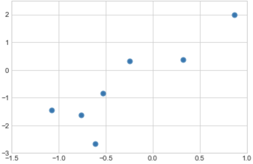
Suppose we got a dataset displayed in a scatterplot like below
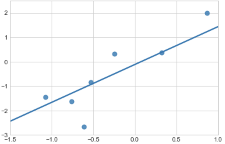
The best fitting line to these data is
There are other possible fitting lines like below
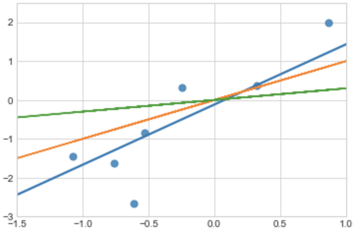
why the blue line is the best line? how can we know(measure) it?
One way to proceed the identification of the best fit is to start measuring the error of data compared to the fitting line.
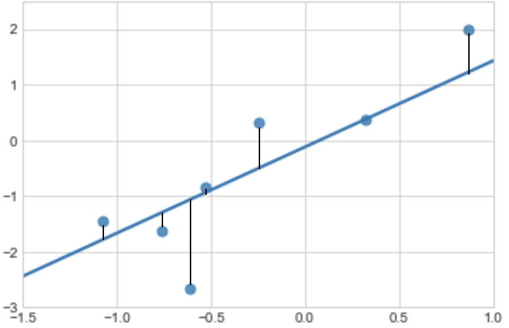
Each data is a dot that has \((X_i,Y_i)\) coordinates. They are the true observations obtained from the true relation equation \(Y_i = \beta_0 + \beta_1 X_i\). The blue fitting line is a linear projection of estimated values obtained from the estimated relation equation \(\hat{Y}_i = \hat{\beta}_0 + \hat{\beta}_1 X_i \). The black segments represent the error we make by substituting \(Y_i\) with \(\hat{Y}_i\), that is
\[Error_i = Y_i - \hat{Y}_i = Y_i - \hat{\beta}_0 - \hat{\beta}_1 X_i\]Note that we have errors because we are trying to find a linear fit to the dataset. Errors do not exist if we do not try to find a linear fit.
Let’s now focus on the error, \( Y_i - \hat{Y}_i \).
We need to get an overall measure of the all errors for each point.
We could think of summing up all the errors like
\[\sum(Y_i - \hat{Y}_i)\]But is this a suitable measure? The answer is no. There are 2 problems.
- Problem 1: A part of errors will be canceled out because some errors are positive and some others are negative;
- Problem 2: We consider that small errors and big errors have the same importance. We might want to penalise big errors.
Solution to Problem 1 and 2
To neutralize the effect of possible cancellations of positive and negative errors, we define the overall error as the Sum of Squared Residuals written as
\[SSR = \sum(Y_i - \hat{Y}_i)^2\]By squaring the error term, we amplify bigger errors. This approach of assessing the error terms is the core idea in Ordinary Least Squares approach of estimating “good” estimates for \(beta_0\) and \(\beta_1\).
2. Ordinary Least Squares (OLS)
We assume thet he size of the mistake is measured by SSR denoted as
\[SSR = \sum^n_{i=1}(Y_i - \hat{Y}_i)^2 = \sum^n_{i=1}\hat{u}^2_i\]and we choose the \(beta_0\) and \(\beta_1\) to have the SSR to be as small as possible. Which means, we want the overall error to be smallest possible.
Formally the problem is written as
\[\min_{\hat{\beta}_0,\hat{\beta}_1} \sum ^n_{i=1}(Y_i - \hat{Y}_i)^2 = \sum^n_{i=1}(Y_i - \hat{\beta}_0 - \hat{\beta}_1 X_i)^2\]By using partial differentiation for each beta, the two necessary first order conditions to identify the solution read as
\[\begin{cases} \beta_0: \frac{\delta \sum^n_{i=1}(Y_i - \hat{\beta}_0 - \hat{\beta}_1 X_i)^2}{\delta \hat{\beta}_0} = 0 \\ \beta_1: \frac{\delta \sum^n_{i=1}(Y_i - \hat{\beta}_0 - \hat{\beta}_1 X_i)^2}{\delta \hat{\beta}_1} = 0 \end{cases}\]these become
\[\begin{cases} \beta_0: -2 \sum^n_{i=1}(Y_i - \hat{\beta}_0 - \hat{\beta}_1 X_i) = 0 \\ \beta_1: -2 \sum^n_{i=1}(Y_i - \hat{\beta}_0 - \hat{\beta}_1 X_i)X_i = 0 \end{cases}\]they give the following solutions
\[\begin{cases} \hat{\beta}_0 = \overline{Y} - \hat{\beta}_1 \overline{X} \\ \hat{\beta}_1 = \frac{\sum(X_i - \overline{X})(Y_i - \overline{Y})}{\sum(X_i - \overline{X})^2} = \frac{Cov(X,Y)}{V(X)} \end{cases}\]Note that \(\overline{X}\) is the mean value of all observed X. It is not the true mean of the population.
Once we have the estimated values of true betas for a given dataset, we can write the OLS fitted line function like
\[\hat{Y}_i = \hat{\beta}_0 + \hat{\beta}_1 X_i\]Remarks
- This OLS fitted line allows us to predict y for any sensible value of x;
- The intercept \(\hat{\beta}_0\) is the predicted y when x = 0. It is often not important and is meaningless to interpret. The most important part is the slope \(\hat{\beta}_1\);
- The slope \(\hat{\beta}_1\) allows us to predict changes in y for any reasonable change in x: \( \Delta \hat{y} = \hat{\beta}_1 \Delta x \);
- If x increases by one unit, then the change in y is caputred by \(\hat{\beta}_1\).
Summary
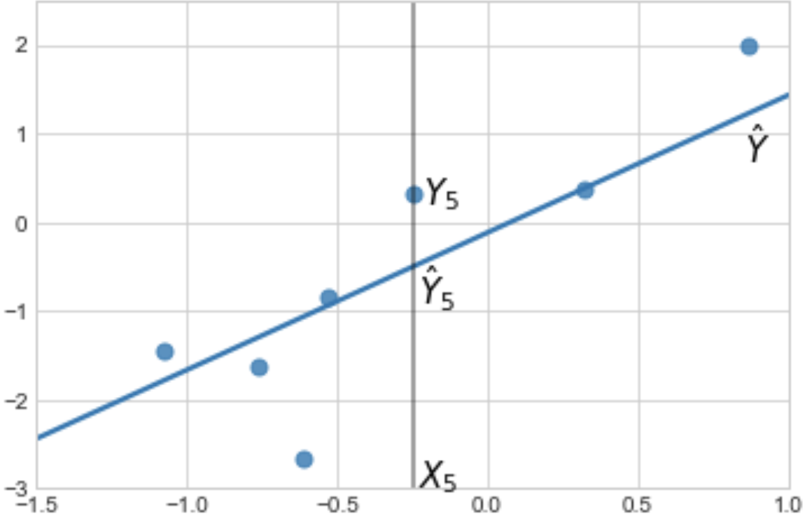
The gap between \(Y_5\) and \(\hat{Y}_5\) is the error, also called residual.
From now, we will focus on \(\hat{\beta}_1\) rather than both \(\hat{\beta}_0\) and \(\hat{\beta}_1\).
2.1 Geometric Interpretation of OLS
2.2 Algebraic Properties of OLS
Let’s consider agian the OLS problem:
\[\min_{\hat{\beta}_0,\hat{\beta}_1} \sum^n_{i=1}(Y_i - \hat{\beta}_0 - \hat{\beta}_1 X_i)^2\]We saw that the two necessary first order conditions are
\[\begin{cases} \beta_0: -2 \sum^n_{i=1}(Y_i - \hat{\beta}_0 - \hat{\beta}_1 X_i) = 0 \\ \beta_1: -2 \sum^n_{i=1}(Y_i - \hat{\beta}_0 - \hat{\beta}_1 X_i)X_i = 0 \end{cases}\]in which constants -2 can be removed because they are irrelevant. We can also replace \((Y_i - \hat{\beta}_0 - \hat{\beta}_1 X_i)\) by the notiation \(\hat{u}_i\). After these two steps, we get:
\[\begin{cases} (1): \sum \hat{u}_i = 0 \\ (2): \sum \hat{u}_i X_i = 0 \end{cases}\]Properties
- First algebraic property (1) tells us that OLS residuals always add up to 0. If the linear fit is perfect, then the sum of residuals must be equal to 0 (in computer simulation it must be extremely close to 0). This doesn’t mean the quality of regression is good, it just means the OLS computation was correctly done;
- Second algebraic property (2) tells us that the sample covariance between residuals \(\hat{u}_i\) and \(X_i\) is 0. This is also called the orthogonality condition.
There are other algebraic properties as well but the properties above are the most important ones.
2.3 Goodness of fit
A consequence of the algebraic properties is the following
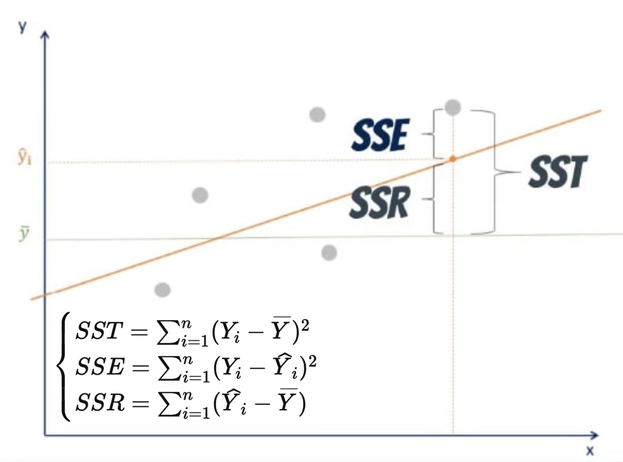
\[\begin{align} SST &= \sum^n_{i=1} (Y_i - \overline{Y})^2 = \sum^n_{i=1} ((Y_i -\widehat{Y}_i) + (\widehat{Y}_i - \overline{Y}))^2 \\ &= \sum^n_{i=1} (Y_i - \widehat{Y}_i)^2 + \sum^n_{i=1} (\widehat{Y}_i - \overline{Y})^2 + 2\sum^n_{i=1}(Y_i -\widehat{Y}_i)(\widehat{Y}_i - \overline{Y}) \\ &= \sum^n_{i=1} (Y_i - \widehat{Y}_i)^2 + \sum^n_{i=1}(\widehat{Y}_i - \overline{Y})^2 \end{align}\]If we define
\[\begin{cases} SST = \sum^n_{i=1} (Y_i - \overline{Y})^2 \\ SSE = \sum^n_{i=1}(Y_i - \widehat{Y}_i)^2 \\ SSR = \sum^n_{i=1}(\widehat{Y}_i - \overline{Y}) \end{cases}\]then we get an equation that says Total Sum of Squares equates the sum of Explained Sum of Squres and Residual Sum of Squares, formally it’s
\[\begin{align} & SST = SSE + SSR \\ & \sum^n_{i=1} (Y_i - \overline{Y})^2 = \sum^n_{i=1}(Y_i - \widehat{Y}_i)^2 + \sum^n_{i=1}(\widehat{Y}_i - \overline{Y}) \end{align}\]Graphically, we can illustrate the equation like below
From this result we can introduce another measure to know how “fit” is our fitted line.
Assuming STT > 0, we can define the faction of the total variation in \(Y_i\) that is explained by \(X_i\) as
\[R^2 = \frac{SSE}{SST} = 1 - \frac{SSR}{SST}\]It can be shown that \(R^2\) is eqaul to the square of the correlation between \(Y_i\) and \(\widehat{Y}_i\). Therefore,
\[0 ≤ R^2 ≤ 1\]- \(R^2 = 0\) means no linear relationship between \(Y_i\) and \(X_i\);
- \(R^2 = 1\) means a perfect linear relationship;
- As \(R^2\) increases, the \(Y_i\) are closer and closer to belonging to the OLS fitted line. Which means our fitted line gaines more and more prediction power;
- But! do not focus to much on the \(R^2\). It is often a useful summary measure but it telles us nothing about causality.
3. Regression
Now that we know what is “fitting”, we have to know what is “regression” Let’s take a practical case to discuss it better.
Let’s frame the case first. On average, people with more schooling earn more than people with less schooling.
-
This connection has an enormous predictive power in spite of the large variation in individual circumstances that sometimes clourds this fact.
-
Of course the fact that more educated people earn more than less educated people does not mean that schooling causes earnings to increase.
-
Even without resolving the causality inssue, it is clear that education predicts earnings in a narrow statistical sense.
3.1 Conditional Expectation Function
The predictive power of regression is summarized by the conditional expectation function(CEF) defined as
\[\begin{align} & E[Y_i|X_i=x] = \int t \cdot f_{Y|X}(t|X_i=x) dt \\ & E[Y_i|X_i=x] = \sum_t t \cdot f _{Y|X}(Y_i=t|X_i=x) \end{align}\]where Y is a dependent variable, X is a vector of covariates and f is a conditional density.
Note that here we are dealing with a population whereas in real life we will be dealing with samples.
3.2 Law of Iterated Expectations
Assume that \(f_{XY}(u,t)\) is joint distribution of \( (X_i,Y_i) \).
The Law of Iterated Expectations says
\[E[Y_i] = E\left[E[Y_i|X_i]\right]\]where the outer expectation uses the distribution of \(X_i\).
This law is useful because it allows to prove the following propositions:
[1] CEF Decomposition Property
The law of iterated expectations implies that
\[\begin{align} Y_i &= CEF + resid. \\ &= E[Y_i|X_i] + \varepsilon_i \end{align}\]where
- Expected value of residual \(\varepsilon_i\) conditional to \(X_i\) is nul:
- \(\varepsilon_i\) is uncorrelated with any function of \(X_i\). Let h(X) be any fnction of X, then:
After CEF decomposition property, we know now that any random variable Y can be decomposed into a piece that is explianed by X, the CEF, and a piece left over which is orthogonal to any function of X.
[2] CEF Prediction Property
This property briefly answers to question “Why is the CEF a good summary of the relationship between Y and X?”.
Let \(m(X_i)\) be any function of X. Then:
\[E[Y_i|X_i] = \arg \min_{m(X_i)} E\left[ (Y_i - m(X_i))^2 \right]\]so the CEF is the Minimum Mean Squared Error (MMSE) predictor of Y given X.
[3] ANOVA Decomposition Property
ANOVA decomposition:
\[V(Y_i) = V(E[Y_i|X_i]) + E[V(Y_i|X_i)]\]where \(V(.)\) denotes the variance and \(V(Y_i/X_i)\) is the conditional variance of Y given X.
75페이지부터 다시 시작