This chapter introduces/reminds you basic statistical concepts and definitions that you must know before learning econometrics.
1. Moments of Distribution
In statistics, we often need to synthetically and algebraically describe the shape of a PDF. In order to do that, we introduce measures that capture different aspects of the shape of a PDF of a random variable.
1.1 Moments?
Before introducing different aspects of the shape of a PDF, you might ask yourself, “why is it called moments?”. This question bothered me for a long time and it still bothers lots of students and even some professors as well. Don’t worry it’s not because we are stupid. It’s because it comes from another science, physics.
In physics, a moment is an expression involving the product of a distance and a physical quantity, and in this way it accounts for how the physical quantity is located or arranged (like mean!!). Moments are usually defined with respect to a fixed reference point. They deal with physical quantities as measured at some distance from that reference point (like variance!!).
Now we know why it’s called moments of distribution. Now let’s move on to the next question: “How many moments are there?”.
1.2 Different moments of distribution
There are four moments that you have to know if you are studying statistics & econometrics.
Let X be a random variable. We can describe PDF(X) with following four moments:
- Mean (1st-order moment): mean, also known as average or expected value, locates the centre of distribution;
- Variance (2nd-order moment): variance, also known as spread, measures variability of X on its distribution. Square root of variance is also often used in statistics and is called standard deviation;
- Skewness (3rd-order moment): skewness measures asymmetry of distribution;
- Kurtosis (4th-order moment): kurtosis measures how thick are tails of distribution. In other words, it measures the likelihood of observing realisations that are far away from the mean.
2. Intuition Behind Moments Measures
In this section, I will try to explain as intuitive as possible why the above four measures are being used in statistics. Detailed mathematical explanation will be followed in the 3rd section.
2.1 Mean
Consider the following dataset D:
\[D = [-3, -1, 1, 2, 2, 5]\]Let’s present them on a line (x-axis):
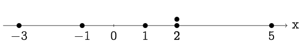
From this graph, we can consider each number in the datatset as a distance from 0. For instance, 5 is physical manifestation of a number by five units. The key point here is that each data has a distance as long as it is different from 0 (We choose 0 because it’s a common reference point but we can very well choose another reference point different from 0).
Therefore, a MEAN meausres the average distance of data in dataset from 0. With the given dataset, we get:
\[\begin{align} \mu &= \frac{\sum^n_{i=1}(x_i - 0)}{n} \\ &= \frac{\sum^n_{i=1}x_i}{n} = 1 \end{align}\]We found that the mean of D is 1. Which means the average distance of data from 0, in the dataset D, is equal to 1.
2.2 Variance
Consider now a new dataset D:
\[D = [1, 1, 1, 1, 1, 1]\]On x-axis:
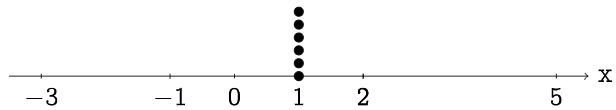
It is evident that D’s mean is 1. But it clearly has a different shape (different spread) of dataset compared to the previous one. This difference in spread is measured by variance:
\[\sigma^2 = \frac{\sum^n_{i=1}(x_i - \mu)}{n}\]This time we do not choose the reference point 0, we choose the mean of the dataset as a reference point.