This chapter introduces/reminds you basic statistical concepts and definitions that you must know before learning econometrics.
1. Random Variable
1.1 Definitions
Simple Definition
Random variable X is a variable whose value is determined by the outcome of a random experiment.
Therefore, a random variable X needs following elements:
- \( x_1, x_2, \cdots, x_k \) (k possible outcomes)
- \( p_1, p_2, \cdots, p_k \) (probability of each outcome)
- \( {x_1, x_2, \cdots, x_k} \) (sample space)
where \(p_i ≥ 0 \) and \( \sum^k_{i=1} p_i = 1 \).
Fancy Definition
In formal mathematical terms, we can also say that a random variable is a function defined on a probability space that maps from the sample space to the real numbers, where
- Probability space \(\equiv (\Omega, \mathcal{F}, \mathbb{P}) \) where
- Sample sapce \(\equiv \Omega \) is a non-empty set of all possible outcomes (numbers) or results (not numbers) from a random experiment.
- \(\sigma\)-algebra \(\equiv \mathcal{F}\) is a set of all possible subsets of \(\Omega\), called events.
- Probability measure \(\equiv \mathbb{P}\) is a function that maps from \(\sigma\)-algebra to a probability \(p \in [0,1]\).
1.2 Random Variable Types
Outcomes of a random variable could either be discrete or continuous. In the first case, the outcomes are numerable. In the second case, the outcomes are not numerable.
2. Probability Distribution Function
For any random variable X one can define its Probability Distribution Function. It is a function of stacked probabilities of each possible value of X when it occurs. There are two types of probability distribution function that are Probability Mass Function and Probability Density Function.
2.1 Probability Mass Function
When X is a discrete random variable, we use Probability Mass Function (pmf). PMF is defined through the following steps:
Let X be a discrete random variable defined as \(X:\Omega \mapsto \mathbb{R} \). Then the probability mass function of X is defined as:
\[\begin{align} pmf(X) \equiv f_X(x) &= P(X=x) \\ &= P(\{\omega \in \Omega: X(\omega) = x\}) \end{align}\]This gives the probability that a discrete random variable X is exactly equal to some value x. You will see right after that this is impossible with continuous random variable.
2.2 Probability Density Function
When X is a continuous random variable, we use Probability Density Function (pdf). The probability density function of X is defind through the following steps:
Let X be a continuous random variable defined as \(X:\Omega \mapsto \mathbb{R} \). Let’s denote the probability density function of X, \(pdf(X) \equiv f_X(x)\). Given this, the probability of X falling within the interval \([a,b]\) is computed by:
\[P(a ≤ X ≤ b) = \int^b_a{f_X(x)dx}\]where \( f_X(x) ≥ 0 \) and \( \int^{+\infty}_{-\infty}{f_X(x)dx} = 1 \).
This gives the probability of X falling within the infinitesimal interval \([a,b]\).
Nota bene:
-
Note that pdf(X) is \(f_X(x)\), not \(\int^b_a{f_X(x)dx}\).
-
Note that the probability of X is exactly equal to a certain value is 0 when X is a continuous RV. Intuitively we know that it’s because we have continuous real numbers that can be infinitesimally refined to extremely and infinitely small numbers. But this explanation does not sound mathematically beautiful.
- Let’s think in this way: the formula above gives the probability of X falling within the interval \([a,b]\). And we know that the integral above gives the area below curve \( f_X(x) \). Trying to find a probability of X is exactly equal to a certain value would mean the probability of X falling within the interval, for instance, \([a,a]\). This is not an area below the curve \(f\). It is a line below the curve \(f\) on the point \(a\). And what is the area of a line? it’s 0. A line has a length, not an area.
3. Cumulative Distribution Function
You now know how to compute probability of X on a certain point (pmf) or on a certain interval (pdf). In addition to that, we can think of computing the sum of probabilities of X before a certain point or after a certain point, by computing the Cumulative Distribution Function (CDF).
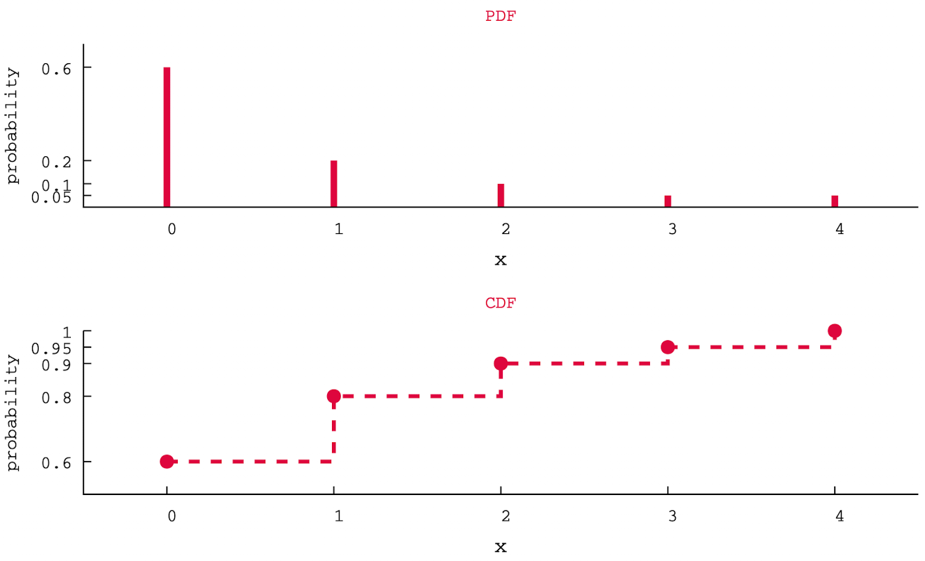
3.1 Discrete random variable
Let X be a discrete random vraiable defined on \(\mathbb{N}\). Cumulative distribution function of X is defined as below:
\[\begin{align} CDF(X) \equiv F_X(x) &= P(X ≤ x) \\ &= \sum_{i=0}P(X=x_i) \\ &= \sum_{i=0}p_i \end{align}\]By definition, CDF(X) is an increasing function of X. In the case of a discrete RV, the shape of CDF function should look like stairs (discontinuous).
Nota bene: for a discrere RV, \(P(X≤x) ≠ P(X< x)\) because unlike contunuous RV, \(P(X=x)\) may not be 0.
Graphical illustration
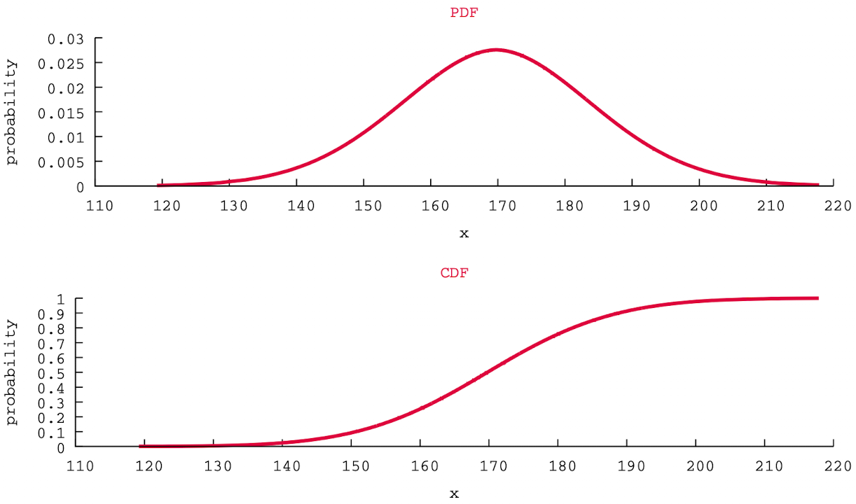
3.2 Contiuous random variable
Let X be a continuous random vraiable. Cumulative distribution function of X is defined as below:
\[\begin{align} CDF(X) \equiv F_X(x) &= P(X ≤ x) = P(X < x) \\ &= \int^x_{-\infty}{f_X(t)dt} \\ &= F_X(b) - F_X(a) \end{align}\]By definition, CDF(X) is an increasing function of X. In the case of a discrete RV, the shape of CDF function should look like a curve (continuous).
Graphical illustration
3.3 Computation Tips
Let X be a continuous random variable. The CDF of X on an arbitrary interval \([a,b]\) is computed by:
CDF on an arbitrary interval
\[P(a≤X≤b) = F_X(b) - F_X(a)\]Probability of X being greater than x
We have only dealt cases where probability of X is being smaller than x. The opposite case, where probability of X being greater then x is computed by:
\[P(X > x) = 1 - F_X(x)\]4. Link between PDF and CDF
Link between PDF and CDF is based on Analysis, which is a branch of mathematics that deals with limits, integration, differentiation etc. Focusing on the relation between integration and differentiation, we can establish the following two relations:
\[\begin{align} F_X(x) &= \int^x_{-\infty}{f_X(t)dt} \\ f_X(x) &= \frac{\delta F_X(x)}{\delta x} \end{align}\]intuitively, one can think of \(f_X(x)\) as being the probability of X falling within the infinitesimal, again, infinitesimal interval \([x,x+\delta x]\).