This is a note for Capital Asset Pricing Model (자본자산 가격결정 모형) and its preliminary work. Since I am very lazy, I am skipping important demonstrations and graphical illustration parts…(sorry) If you find any error, please do let me know at gunhoqw20@gmail.com.
1. Portfolio Composition
The title seems it has a relation with Pr Markowitz’s Portfolio Selection Theory but well… it does not (slightly yes because he basically founded everything).
4 steps:
-
Suppose two financial assets (shares, bonds etc) A and B. They are in the same portfolio and being invested on the same arbitrary period generating stochastic (fancy word for random) returns \(R_A\) and \(R_B\).
-
Suppose we invest a unit of investment \(I\) (let’s say I = 1$) which has following allocations: \(x\), proportion for A, and \((1-x)\), proportion for B. Let’s call future values of shares A and B as \(V_A\) and \(V_B\).
-
Returns of \(R_A\) and \(R_B\) are determined by:
\[\begin{align} R_A &= V_A - 1 \\ R_B &= V_B -1 \end{align}\]Therfore, the return of entire portolio is:
\[\begin{align} R_P &= (xV_A + (1-x)V_B) -1 \\ R_P &= xR_A + (1-x)R_B \end{align}\] -
Since \(R_A\) and \(R_B\) are both random variables, they both have fisrt-order moment (mean denoted as \(\mu_i\) or \(E(R_i)\)) and second-order moment (variance denoted as \( \sigma ^2_i \) or \( V(R_i) \)). In consequence, \(R_P\) is also a random variable that has mean, variance, and covariance (denoted as \( \sigma _{ij} \)). This gives the formulae below:
or
\[\begin{align} \mu_P &= x\mu_A + (1-x)\mu_B \\ \sigma^2_P &= x^2\sigma^2_A + (1-x)^2\sigma^2_B + 2x(1-x)\sigma_{AB} \end{align}\]From these formulae, we can have two simple types of portfolio:
- Portfolio containing a risky asset and a non-risky asset;
- Portfolio containing two risky assets
2. Portfolio: one risky asset and one non-risky asset
Let A a risky asset and B a non-risky asset attached to a risk-free rate \( r_f \). If we apply such composition to previous formula, we get: (Don’t forget that we are only investing 1$ still)
\[\begin{align} E(R_P) &= xE(R_A) + (1-x)r_f \\ V(R_P) &= \sigma^2_P = x^2 \sigma^2_A \end{align}\]From \(V(R_P)\), we get the following allocation:
\[x = \frac{\sigma_P}{\sigma_A}\]from which we can rewrite the expected portfolio return formula as following:
\[\begin{align} E(R_P) &= \frac{\sigma_P}{\sigma_A} E(R_A) + (1-\frac{\sigma_P}{\sigma_A})r_f \\ &= \frac{\sigma_P}{\sigma_A}(E(R_A)-r_f) + r_f \end{align}\]Finally with some rearrangement, we get:
\[E(R_P) = \frac{E(R_A)-r_f}{\sigma_A}\sigma_P + r_f\]We remark two things from this equation:
- \(E(R_P)\) is a linear function of risk (\(\sigma_P\)) with risk free rate \(r_f\) as y-intercept.
- The slope of this function is called Sharpe ratio which is interpreted as excessive return of share A per each unit of risk undertakend by the share A.
3. Portfolio: two risky assets
Let A and B two different risky assets. We apply the same logic. Then the formula becomes (or stays as):
\[\begin{align} E(R_P) &= xE(R_A) + (1-x)E(R_B) \\ V(R_P) &= x^2\sigma^2_A + (1-x)^2\sigma^2_B + 2x(1-x)\sigma_{AB} \end{align}\]In this case, the capital allocation line is no longer linear except a particular case when A and B are perfectly and positively correlated. The correlation proxy \(\rho _{AB}\) is computed by:
\[\rho_{AB} = \frac{Cov(R_A,R_B)}{SD(A) \times SD(B)} = \frac{\sigma_{AB}}{\sigma_A \sigma_B}\]where \(\sigma _{AB}\) can be either negative or positive (nul is impossible in real life).
We can find the optimal allocation proportion \(x\) by first-order condition of utility function of the portfolio which I will not discuss here. And from the optimal allocation \(x\), we generalise the portfolio to \(n\) risky assets then we should be able to draw tangent portfolio, efficient frontier (see the work of Eugene Fama), feasible set etc.
4. Markowitz Optimisation Problem
Let’s assume we did a great job in analysing efficient frontier and feasible set ;D
Then it rises the following problem proposed by Harry Markowitz: agents want to maximize their expected return of portolio composed by \(n\) different shares hence \(n\) different allocations \(x_i\) such that \( \sum^n_{i=1} x_i = 1 \), with a target level of risk \( \tilde{\sigma}^2_P \).
Mathematical formulation of the problem: (u/c means under constraint, equally we say subject to)
\[\begin{cases} \max_{x_i} E(R_P) = \sum^n_{i=1} x_i E(R_i) \\ u/c: \sum^n_{i=1}\sum^n_{j=1}x_ix_i\sigma_{ij} = \tilde{\sigma}^2_P \\ u/c: \sum^n_{i=1}x_i = 1 \end{cases}\]which can be reformulated as below:
\[\begin{cases} \min_{x_i} \sigma^2_P = \sum^n_{i=1}\sum^n_{j=1}x_ix_i\sigma_{ij} \\ u/c: \sum^n_{i=1} x_i E(R_i) = \tilde{E}(R_P) \\ u/c: \sum^n_{i=1}x_i = 1 \end{cases}\]From this formulation of allocation optimisation problem (basically portfolio diversification problem), Sharpe, Mossin, and Lingtner start modelising the first version of CAPM called Sharpe-Mossin-Lintner CAPM.
5. Sharpe-Mossin-Lintner CAPM
This model, that I will call Sharpe CAPM from now on, allows us to determine the price of financial assets at any moment.
5.1 Hypotheses of the model
- All investors are more or less averse to risk > kinda true
- All investors have the same time horizon for investment > unrealistic
- All investors are addressing to the same problem that is Markowitz Problem:
- only way to diversify is to change the allocations
- all investors anticipate same expected return (gain) and same variance (risk) of portfolio
- Financial market is a perfect market:
- no tax
- no transaction cost
- no asymmetry of information
- there is a risk-free asset with \(r_f\) at which we can borrow and lend capital freely
All these look quite heavy but what you gotto know are two things: Markowitz problem is in the center, and there is a risk-free asset.
5.2 Sharpe-CAPM Formula Induction
Preliminary Step
Let’s bring back the Markowitz problem but with a risk-free rate \(r_f\). The problem is now written as below:
\[\begin{cases} \min_{x_i} \sigma^2_P = \sum^n_{i=1}\sum^n_{j=1}x_ix_i\sigma_{ij} \\ u/c: \sum^n_{i=1} x_i E(R_i) + x_0r_f = E(R_P) \\ u/c: \sum^n_{i=1}x_i + x_0 = 1 \end{cases}\]We combine two constraints into one. From the second constraint, we get \( x_0 = 1 - \sum x_i \). Put it into the first contraint:
\[\begin{align} &E(R_P) = \sum x_i E(R_i) + (1-\sum x_i)r_f \\ &E(R_P) - r_f = \sum x_i E(R_i) - r_f\sum x_i + r_f - r_f \\ &E(R_P) - r_f = \sum x_i (E(R_i) - r_f) \end{align}\]The last equation means (excess of portfolio return) = (sum of each expected return of risky asset diminshed by risk-free return). This result is quite intuitive yet hard to be proven arithematically. The queation can be transformed into matrix as well.
Let \(V\), var-cov matrix of all returns of size (N,N) and all other terms are as below
\[\mathbb{R} = \begin{bmatrix} R_1 \\ \vdots \\ R_n \end{bmatrix} ~~~ E = \begin{bmatrix} E(R_1) - r_0 \\ \vdots \\ E(R_n) - r_0 \end{bmatrix} ~~~ X = \begin{bmatrix} X_1 \\ \vdots \\ X_n \end{bmatrix}\]Optimisation(minimisation) problem of investors can be written as
\[\begin{cases} \min_X X^T V X \\ u/c: X^T E = E(R_P) - r_f \end{cases}\]Lagrangian optimisation:
\[\mathcal{L}(X,\lambda) = X^T V X + \lambda(E(R_P)-r_f-X^TE)\]First Order Condition:
\[\frac{\delta \mathcal{L}}{\delta X} = 0 ~~~ \iff ~~~ 2VX - \lambda E = 0\] \[X^* = \frac{1}{2}\lambda V^{-1} E\]This X matrix is the vector of all optimal allocations taking Sharpe ratio as its slope. This is true for all investors.
And at Equilibirum, the sum of all portfolios of investors must be equal to the market portfolio. In other words, at equlibirum, the total demand of financial assets is equal to the total supply of financial assets on financial market. Given this parity, at equilibrium, the optimal allocation X can be summed up from both supply and demand thus can be rewritten as
\[X_M = \lambda_M V^{-1} E\]where \(\lambda _M \) is unknown.
This relation contains both first-order moment and second-order moment anticipations of investors. We now have to determine what is this unknown \(\lambda _M \).
First Big Step:
- Isolate E.
- Multiply \(X^T\) at both sides.
- Focus on the market return excess \(E(R_M) - r_f \). Also, \(X^T_M X\) will add up to 1. Therefore, \(X^T_M V X_M \) is equal to market volatility which is \(\sigma ^2_M\):
- Finally we isolate \(\lambda _M \)
We found an expression for \(\lambda _M \).
Second Big Step:
- Going back to the first big step, we isolate E, but only for a single financial asset \(i\).
- We replace \(\lambda _M \) by the result of the First Big Step:
5.3 Sharpe CAPM Formula
With some arrangement we get
\[E(R_i) - r_f = \frac{\sigma_{iM}}{\sigma^2_M}(E(R_P)-r_f)\]or we can also write
\[E(R_i) = \frac{\sigma_{iM}}{\sigma^2_M}(E(R_P)-r_f) + r_f\]There is no difference between the two formlae above. Conventionally people tend to use more the first one. One of few reasons is that it is simpler to draw a graph since there is no y-intercept whereas the second formula does have y-intercept which is \(r_f\). It is although the same.
Most importantly from the formula, we remark that it’s a linear function. And this equality relation (or equation) is called fundamental relation of CAPM, or fundamental equation of CAPM.
5.4 Interpretation
We can simplify the formula once more by replacing the slope by Beta ratio.
\[E(R_i) - r_f = \beta_i(E(R_P)-r_f)\]- \( E(R_P)-r_f \) can be interpreted as risk premium proportional to \(\beta _{i}\).
- \(\beta_{i} = \frac{\sigma_{iM}}{\sigma^2_M} \) can be interpreted in two ways:
- sensivity of asset \(i\) in regards to market: If Beta of share \(i\) is 2,00 then when market value goes up by 1,00%, share value of \(i\) will go up by 2,00%. This means \(i\) is positively very sensitive to market.
- contribution of asset \(i\) to risk of the market:
- If \(\sigma_{iM}\) > \( \sigma ^2_{M} \), then owning the share accelerates the risk of the market;
- If \(\sigma_{iM}\) < \( \sigma ^2_{M} \), then owning the share slows down the risk of the market.
(Often we denote \(\beta_i\), \(\beta_{iM}\) to remind it is correlated with market volatiliy)
5.5 Model Expansion
We can expand the model from a single asset to a portfolio.
For a portfolio \(P\),
\[\beta_{P} = \sum^n_{i=1}x_{Pi} \beta_{iM} = \frac{\sigma_{PM}}{\sigma^2_M}\]Therefore expected return of portfolio return is
\[E(R_P)-r_f = \beta_{P}(E(R_M)-r_f)\]5.6 Limits
We said two key assumptions of Sharpe-CAPM are “Markowitz Problem” and “Existence of risk-free asset at which agents can lend and borrow”. The latter is actually unrealistic well… impossible! We need another model that does not need that second assumption.
6. Black-CAPM
Fischer Black himself identifies four key assumptions in Sharp-Mossin-Lintner CAPM in his paper “Capital Market Equilibrium with Restricted Borrowing” on JSTOR journal:
6.1 Previous Hypotheses
- All investors have the same opinions about the possibilities of various end-of-period values for all assets. They have a common joint probability distribution for the returns on the available assets.
- The common probability distribution describing the possible returns on the available assets is joint normal (or joint stable with a single characteristic exponent).
- Investors choose portfolios that maximize their expected end-of-period utility of wealth, and all investors are risk averse. (Every investor’s utility function on end-of-period wealth increases at a decreasing rate as his wealth increases.)
- An investor may take a long or short position of any size in any asset, including the riskless asset. Any investor may borrow or lend any amount he wants at the riskless rate of interest.
6.2 Black-CAPM Hypotheses
Lintner has shown that removing the first assumption does not change the structure of capital asset prices in any significant way, and second and third assumptions are generally regarded as acceptable approximations to reality. Nevertheless, Black finds the 4th assumption the most restrictive amongst all, and is not a very good approximation for many investors, and one feels that the model would be changed substantially if this assumption were dropped.
Also, Black, Jensen, and Scholes analyzed the returns on portfolios of stocks at different levels of \(\beta_i\) in the 1926-1966 period. They found that the average returns on these portfolios are not consistent with the fundamental equation of CAPM developed by Sharpe.
Black starts constructing his new model by assuming that investors may take long or short positions of any size in any risky asset, but that there is no riskless asset and that no borrowing or lending at the riskless rate of interest is allowed.
6.3 Black-CAPM Formula Induction
Preliminary Step
Since there is no risk-free asset, Markowitz problem in this situation writes as
\[\begin{cases} \min_{x_i} \sigma^2_P = \sum^n_{i=1}\sum^n_{j=1}x_ix_i\sigma_{ij} \\ u/c: \sum^n_{i=1} x_i E(R_i) = E(R_P) \\ u/c: \sum^n_{i=1}x_i = 1 \end{cases}\]In matrix form, we get
\[\mathbb{R} = \begin{bmatrix} R_1 \\ \vdots \\ R_n \end{bmatrix} ~~~ E = \begin{bmatrix} E(R_1) \\ \vdots \\ E(R_n) \end{bmatrix} ~~~ X = \begin{bmatrix} X_1 \\ \vdots \\ X_n \end{bmatrix} ~~~ \mathbb{1} = \begin{bmatrix} 1 \\ \vdots \\ 1 \end{bmatrix}\]The problem then can be rewritten as
\[\begin{cases} \min_X X^TVX \\ u/c: X^TE = E(R_P) \\ u/c: X^T \mathbb{1} = 1 \end{cases}\]Langrangian Optimisation:
\[\mathcal{L}(X,\lambda,\gamma) = X^T V X + \lambda(E(R_P)-X^TE) + \gamma(1-X^T\mathbb{1} )\]First Order Condition:
\[\begin{align} \frac{\delta \mathcal{L}}{\delta X} = 0 ~~~ &\iff ~~~ 2VX - \lambda E - \gamma \mathbb{1} = 0 \\ &\iff ~~~ X = \frac{1}{2} V^{-1} (\lambda E + \gamma \mathbb{1}) \\ &\iff ~~~ X^* = \frac{1}{2} \lambda V^{-1} E + \frac{1}{2} \gamma V^{-1} \mathbb{1} \end{align}\]Again, at equilibrium, we get
\[X_M = \lambda_M V^{-1} E + \gamma_M V^{-1} \mathbb{1}\]This is the optimal allocation matrix. This time, we got two unknown paramters \(\lambda_M\) and \(\gamma_M\)
First Big Step
- Isolate E.
- Multiply \(X^T_M \) at both sides.
where \( X^T_M \mathbb{1} = 1 \)
- Focus on the market return \(E(R_M)\). Also, \(X^T_M X\) will add up to 1. Therefore, \(X^T_M V X_M \) is equal to market volatility which is \(\sigma ^2_M\). Given these, we get:
Remark: we have (marginal market revenue) = (marginal cost) relation
- We can reduce the size of equation from market to a portfolio
- This step is the key part. Black introduces a particular case of a portfolio whose beta is zero. Zero-beta portfolio can be expressed as such
With the same intution used in the step right before, the expected return of zero-beta portfolio Z can be written as
\[\begin{align} \lambda_M E(R_Z) &= \sigma_{ZM} - \gamma_M \\ &= - \gamma_M \end{align}\] \[D \equiv MR = \lambda_M E(R_Z) + \gamma_M = 0\]This is the marginal revenue of investors(consumers) in this particular portfolio. Allow me to remind you that in economics, in a competitive market, marginal revenue is equal to the total demand curve. Also, in the same type of market, marginal cost is equal to the total supply curve. As we saw two steps before, marginal cost is
\[S \equiv MC = \lambda_M E(R_M) - \sigma^2_M + \gamma_M = 0\]Second Big Step:
- Let’s now establish the equilibrium between D and S:
Result 1
\[\sigma^2_M = \lambda_M(E(R_M) - E(R_Z))\]- Let’s recall the following relation:
We can reduce this to a single asset,
\[\begin{align} &\lambda_M E(R_i) = \sigma_{iM} - \gamma_M \\ \iff~~~& \lambda_M E(R_i) - \sigma_{iM} + \gamma_M = 0 \\ \iff~~~& \lambda_M E(R_i) - (\sigma_{iM} - \gamma_M) = 0 \end{align}\]At equilibrium, the result above should be equal to the same result but sized up to the entire market,
\[\begin{align} & \lambda_M E(R_i) - (\sigma_{iM} - \gamma_M) = \lambda_M E(R_M) - (\sigma^2_{M} - \gamma_M) \\ \iff~~~& (\sigma^2_{M} - \sigma_{iM}) = \lambda_M (E(R_M) - E(R_i)) \\ \iff~~~& \frac{1}{\lambda_M} = \frac{E(R_M) - E(R_i)}{\sigma^2_{M} - \sigma_{iM}} \end{align}\]Result 2
\[\frac{1}{\lambda_M} = \frac{E(R_M) - E(R_i)}{\sigma^2_{M} - \sigma_{iM}}\]At this stage, we have successfully removed \(\gamma_M\) and found an expression for \(\lambda_M \).
- Plug in the Result 1 into the Result 2:
Result 1:
\[\sigma^2_M = \lambda_M(E(R_M) - E(R_Z)\]Result 2:
\[\frac{1}{\lambda_M} = \frac{E(R_M) - E(R_i)}{\sigma^2_{M} - \sigma_{iM}}\]We get
\[\frac{E(R_M) - E(R_i)}{\sigma^2_{M} - \sigma_{iM}} = \frac{E(R_M) - E(R_Z)}{\sigma^2_M}\]After multiple arrangements, we shall get
\[E(R_i) - E(R_Z) = \frac{\sigma_{iM}}{\sigma^2_M}(E(R_M) - E(R_i))\]Now we have the formula.
6.4 Black-CAPM Formula
We found
\[E(R_i) - E(R_Z) = \frac{\sigma_{iM}}{\sigma^2_M}(E(R_M) - E(R_i))\]Which can be again simplified with Beta ratio
\[E(R_i) - E(R_Z) = \beta_i(E(R_M) - E(R_i))\]Quoting from Black’s interpretation, this is “the expected return on every asset, even when there is no riskless asset and riskless borrowing is not allowed, is a linear function of its \(\beta\).”
Here, we see that the introduction of a riskless asset simply replaces \(E(R_Z)\) with \(r_f\).
6.5 Graphical Illustration
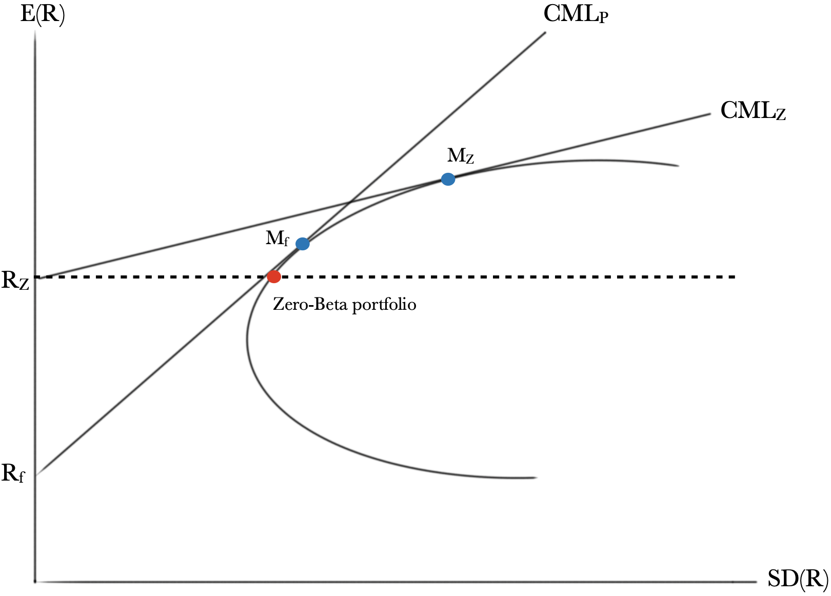
Reminder:
\[CML_f:~ E(R_{P})= \frac{E(R_M)-R_f}{\sigma _M}\sigma _{P} + R_f\]- We call CML that is tangent to efficient frontier, Capital Allocation Line (CAL)
- We can also draw a Security Market Line:
This is not any sort of CML. It is completely different. It takes beta as x-axis.
Interpretation:
In theory, people can borrow money at safe rate \(r_f\) (capital R in the picture). Riskless asset’s tangent portfolio at \(M_f\) is the best way to borrow and invest for those agents who borrowed money at \(r_f\). But in reality, there is no such thing as safe rate nor the risk free loan. That is why zero-Beta asset’s capital market line (CML) is above the riskless asset’s CML and is less steeper. We can also see that zero-Beta asset’s tangent portfolio \(M_Z\) is located on the right-hand side of riskless tangent portfolio on the same efficient frontier. This simply means it has more risk (x-axis is \(\sigma\) which means risk) hence greater expected return. In the presence of both assets (zero-Beta and riskless), all rational investors (borrowers) should choose any protfolio between \(M_f\) and \(M_Z\), depending on their degree of risk aversion.